ACCA考官文章(F5)THE LEARNING RATE AND LEARNING EFFECT
Under the new exam structure for Paper F5, learning curves will continue to be examined, the only change being that questions may vary a little bit more than they have done in the past.
The December 2013 syllabus reads ‘estimate the learning effect and apply the learning curve to a budgetary problem, including calculations on steady states.’ Thus far, this has been interpreted to mean that the learning rate will always be given in a question and questions will focus purely on 'estimating the learning effect' – that is, calculating the labour time and usually cost for a given process. Historically, the requirements of questions have been such it has been necessary for candidates to use the algebraic method, applying the learning curve formula to problems, rather than the tabular approach.
Both methods, however, have actually been examinable under the syllabus, and for teaching purposes, the tabular approach is always a good starting point to demonstrate how the learning curve effect actually works.
In the syllabus for December 2014 onwards, the words ‘learning rate and learning effect’ will be used rather than simply ‘learning effect’. This wording has been changed in order to make it clear that candidates could now be asked to calculate learning rates too.
The purpose of this article is, however, twofold: first, it is to summarise the history of the learning curve effect and help candidates understand why it is important. Second, it is to look at what past learning curve questions have required of candidates and to clarify how future questions may go beyond this.
A BRIEF HISTORY OF THE LEARNING CURVE
In practice, it is often found that the resources required to make a product decrease as production volumes increase. It costs more to produce the first unit of a product than it does to produce the one hundredth unit. In part, this is due to economies of scale since costs usually fall when products are made on a larger scale. This may be due to bulk quantity discounts received from suppliers, for example. The learning curve, effect, however, is not about this; it is not about cost reduction. It is a human phenomenon that occurs because of the fact that people get quicker at performing repetitive tasks once they have been doing them for a while. The first time a new process is performed, the workers are unfamiliar with it since the process is untried. As the process is repeated, however, the workers become more familiar with it and better at performing it. This means that it takes them less time to complete it.
The first reported observation of the learning curve goes as far back as 1925 when aircraft manufacturers observed that the number of man hours taken to assemble planes decreased as more planes were produced. TP Wright subsequently established from his research of the aircraft industry in the 1920s and 1930s that the rate at which learning took place was not random at all and that it was actually possible to accurately predict how much labour time would be required to build planes in the future. During World War II, US government contractors then used the learning curve to predict cost and time for ship and plane construction. Gradually, private sector companies also adopted it after the war.
The specific learning curve effect identified by Wright was that the cumulative average time per unit decreased by a fixed percentage each time cumulative output doubled. While in the aircraft industry this rate of learning was generally seen to be around 80%, in different industries other rates occur. Similarly, depending on the industry in question, it is often more appropriate for the unit of measurement to be a batch rather than an individual unit.
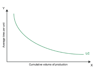
The learning process starts as soon as the first unit or batch comes off the production line. Since a doubling of cumulative production is required in order for the cumulative average time per unit to decrease, it is clearly the case that the effect of the learning rate on labour time will become much less significant as production increases. Eventually, the learning effect will come to an end altogether. You can see this in Figure 1 below. When output is low, the learning curve is really steep but the curve becomes flatter as cumulative output increases, with the curve eventually becoming a straight line when the learning effect ends.
Figure 1
The learning curve effect will not always apply, of course. It flourishes where certain conditions are present. It is necessary for the process to be a repetitive one, for example. Also, there needs to be a continuity of workers and they mustn’t be taking prolonged breaks during the production process.
THE IMPORTANCE OF THE LEARNING CURVE EFFECT
Learning curve models enable users to predict how long it will take to complete a future task. Management accountants must therefore be sure to take into account any learning rate when they are carrying out planning, control and decision-making. If they fail to do this, serious consequences will result. As regards its importance in decision-making, let us look at the example of a company that is introducing a new product onto the market. The company wants to make its price as attractive as possible to customers but still wants to make a profit, so it prices it based on the full absorption cost plus a small 5% mark-up for profit. The first unit of that product may take one hour to make. If the labour cost is $15 per hour, then the price of the product will be based on the inclusion of that cost of $15 per hour. Other costs may total $45. The product is therefore released onto the market at a price of $63. Subsequently, it becomes apparent that the learning effect has been ignored and the correct labour time per unit should is actually 0.5 hours. Without crunching through the numbers again, it is obvious that the product will have been launched onto the market at a price which is far too high. This may mean that initial sales are much lower than they otherwise would have been and the product launch may fail. Worse still, the company may have decided not to launch it in the first place as it believed it could not offer a competitive price.
Let us now consider its importance in planning and control. If standard costing is to be used, it is important that standard costs provide an accurate basis for the calculation of variances. If standard costs have been calculated without taking into account the learning effect, then all the labour usage variances will be favourable because the standard labour hours that they are based on will be too high. This will make their use for control purposes pointless.
Finally, it is worth noting that the use of learning curve is not restricted to the assembly industries it is traditionally associated with. It is also used in other less traditional sectors such as professional practice, financial services, publishing and travel. In fact, research has shown that just under half of users are in the service sector.
HOW LEARNING CURVES HAVE BEEN EXAMINED IN THE PAST
The learning curve effect has regularly been examined in Paper F5. For example, in December 2011, it was examined in conjunction with life cycle costing. Candidates were asked to calculate a revised lifecycle cost per unit after taking into account the learning effect. This involved working out the incremental labour time taken to produce the final 100th unit made before the learning effect ended. This is a fairly common exam requirement which tests candidates’ understanding of the difference between cumulative and incremental time taken to produce a product and the application of the learning curve formula. It is worth mentioning at this point that you should never round learning curve calculations to less than three decimal places. In some questions, where the learning effect is small, over-rounding will lead to a candidate wiping out the entire learning effect and then the question becomes pointless.
The learning curve formula, as shown below, is always given on the formula sheet in the exam.
Y = axb
Where Y = cumulative average time per unit to produce x units
a = the time taken for the first unit of output
x = the cumulative number of units produced
b = the index of learning (log LR/log2)
LR = the learning rate as a decimal
While a value for ‘b’ has usually been given in past exams there is no reason why this should always be the case. All candidates should know how to use a scientific calculator and should be sure to take one into the exam hall.
In June 2013, the learning effect was again examined in conjunction with lifetime costing. Again, as has historically been the case, the learning rate was given in the question, as was the value for ‘b’.
Back in June 2009, the learning curve effect was examined in conjunction with target costing. Once again, the learning rate was given, and a value for ‘b’ was given, but this time, an average cost for the first 128 units made was required. It was after this point that the learning effect ended, so the question then went on to ask candidates to calculate the cost for the last unit made, since this was going to be the cost of making one unit going forward in the business.
It can be seen, just from the examples given above, that learning curve questions have tended to follow a fairly regular pattern in the past. The problem with this is that candidates don’t always actually think about the calculations they are performing. They simply practise past papers, learn how to answer questions, and never really think beyond this. In the workplace, when faced with calculations involving the learning effect, candidates may not be able to tackle them. In the workplace, the learning rate will not be known in advance for a new process and secondly, even if it has been estimated, differences may well arise between expected learning rates and actual learning rate experienced. Therefore, it seemed only right that future questions should examine candidates’ ability to calculate the learning rate itself. This leads us on to the next section of the article.
HOW THE LEARNING EFFECT AND LEARNING RATES MAY BE EXAMINED FROM DECEMBER 2014 ONWARDS
Obviously, the learning effect could be examined exactly as it has been in past exams, with candidates being asked to calculate the time taken to produce an individual unit or a number of units of a product either when the learning curve is still in effect or when it has ended. This objective of the syllabus has not changed. As mentioned earlier, historically, questions have required the use of the algebraic method and a value for ‘b’ has usually been given in the exam. Moving forward, since calculations of the learning rate itself may be required in future exams, it becomes even more important that candidates are familiar with both the tabular method and using their scientific calculators. The following question is an example of the kind of question that may appear in future exams. Here, the tabular method is the simplest way to answer the question.
Example 1
P Co operates a standard costing system. The standard labour time per batch for its newest product was estimated to be 200 hours, and resource allocation and cost data were prepared on this basis.
The actual number of batches produced during the first six months and the actual time taken to produce them is shown below:
| Month | Incremental number of batches produced each month | Incremental labour hours taken to produce the batches |
|---|---|---|
| June | 1 | 200 |
| July | 1 | 152 |
| August | 2 | 267.52 |
| September | 4 | 470.8 |
| October | 8 | 1,090.32 |
| November | 16 | 2,180.64 |
Required
(a) Calculate the monthly learning rate that arose during the period.
(b) Identify when the learning period ended and briefly discuss the implications of this for P Co.
Solution
(a) Monthly rates of learning
| Month | Incremental number of batches | Incemental total hours | Cumulative number of batches | Cumulative total hours | Cumulative average hours per batch | |
|---|---|---|---|---|---|---|
| June | 1 | 200 | 1 | 200 | 200 | |
| July | 1 | 152 | 2 | 352 | 176 | |
| August | 2 | 267.52 | 4 | 619.52 | 154.88 | |
| September | 4 | 470.8 | 8 | 1090.32 | 136.29 | |
| October | 8 | 1090.32 | 16 | 2180.64 | 136.29 | |
| November | 16 | 2180.64 | 32 | 4361.28 | 136.29 |
Learning rate:
176/200 = 88%
154.88/176 = 88%
136.29/154.88 = 88%
Therefore the monthly rate of learning was 88%.
(b) End of learning rate and implications
The learning period ended at the end of September. This meant that from October onwards the time taken to produce each batch of the product was constant. Therefore, in future, when P Co makes decisions about allocating its resources and costing the product, it should base these decisions on the time taken to produce th eighth batch, which was the last batch produced before the learning period came to an end. The resource allocations and cost data prepared for the last six months will have been inaccurate since they were based on a standard time per batch of 200 hours.
P Co could try and improve its production process so that the learning period could be extended. It may be able to do this by increasing the level of staff training provided. Alternatively, it could try to incentivise staff to work harder through payment of bonuses, although the quality of production would need to be maintained.
Example 2
The first batch of a new product took six hours to make and the total time for the first 16 units was 42.8 hours, at which point the learning effect came to an end.
Calculate the rate of learning.
Solution
Again, the easiest way to solve this problem and find the actual learning rate is to use a combination of the tabular approach plus, in this case, a little bit of maths. There is an alternative method that can be used that would involve some more difficult maths and use of the inverse log button on the calculator, but this can be quite tricky and candidates would not be expected to use this method. Should they choose to do so, however, full marks would be awarded, of course.

Using algebra:
Step 1: Write out the equation:
42.8 = 16 x (6 x r4)
Step 2: Divide each side by 16 in order to get rid of the ’16 x’ on the right hand side of the equation:
2.675 = (6 x r4)
Step 3: Divide each side by 6 in order to get rid of the ‘6 x’ on the right hand side of the equation:
0.4458333 = r4
Step 4: take the fourth root of each side in order to get rid of the r4 on the right hand side of the equation. You should have a button on your calculator that says r4 or x1/y. Either of these can be used to find the fourth root (or any root, in fact) of a number. The key is to make sure that you can use your calculator properly before you enter the exam hall rather than trying to work it out under exam pressure. You then get the answer:
r = 0.8171
This means that the learning rate = 81.71%.
SUMMARY
The above two examples demonstrate the type of requirements that you may find in future questions on learning curves, together with the old-style requirements that have traditionally been found in past questions in Paper F5. Remember: nothing new is being added to the syllabus here. All that we are doing is encouraging you to think a little and, in some case, perhaps use a little bit of the maths that, as a trainee accountant, you should be more than capable of applying.





 白金級認(rèn)可培訓(xùn)資質(zhì)(總部)
 課程試聽
課程試聽
 職業(yè)規(guī)劃
 ACCA中文教材
 考位預(yù)約
 免費(fèi)資料




 題庫下載
題庫下載
 模擬機(jī)考




 CFA?成績查詢




 GARP協(xié)會(huì)官方認(rèn)可FRM?備考機(jī)構(gòu)

